Brunner-Munzel 検定の効果量と Cohen の d
井口豊(生物科学研究所,長野県岡谷市)
最終更新: 2022 年 11 月 20 日
1. はじめに
Brunner-Munzel 検定は,正規分布かどうか,等分散かどうか,それを気にせずに適用される検定である。しかし,その効果量の計算については,あまり解説が無い。ここでは,統計ソフト R を利用して,シミュレーションを含めて解説する。
2. Brunner-Munzel 検定の効果量の定義
ここでは, Mann-Whitney U 検定(Wilcoxon 順位和検定)の検定統計量 W を知っているという前提で, R を利用して, Brunner-Munzel 検定の効果量の定義を示す。 W については,別ページを参照してほしい(Mann-Whitney U 検定の統計量: R による注意点)。
まず, R による U 検定の計算用に, wilcox.test 関数がある。これを使って計算すると,検定統計量 W が表示される。この W を使って, Brunner-Munzel 検定の効果量 Stochastic superiority, S は以下のように表される。
ここで, n1, n2 は,検定対象となった 2 群それぞれの標本サイズである。
この効果量の数値は, R のパッケージ lawstat の中の brunner.munzel.test 関数を使ったときに, estimate という項目で出力される。
brunner.munzel.test 関数のマニュアルで, Value 項目の中の estimate を見ると,以下のように書いてある。
an estimate of the effect size
文字通り,これが Brunner-Munzel 検定の効果量であり, Stochastic superiority とも呼ばれる統計量である。
前述の W を使った定義式と,この estimate の数値が一致するか,乱数のデータを使ってシミュレーションで調べてみよう。以下のようなスクリプトで計算した。
#############
library(lawstat)

es<- replicate(100, {
  nx<- sample(5:15, size = 1)
  ny<- sample(5:15, size = 1)

  x<- sample(1:20, size = nx, replace = T)
  y<- sample(1:20, size = ny, replace = T)

  w<- wilcox.test(x, y)$statistic

  c(
   (nx*ny - w)/(nx*ny),
   brunner.munzel.test(x, y)$estimate
   )
})

par(oma = c(3, 3, 2, 2))

plot(
  es[1, ], es[2, ],
  xlab = "(nx * ny - w) / (nx * ny)",
  ylab = "brunner.munzel.test(x, y)$estimate",
  cex.lab  = 1.5,
  cex.axis = 1.5,
  col = "red",
  main = "Stochastic superiority"
)

abline(0, 1)

##################
結果は,以下の図 1 のようになった。
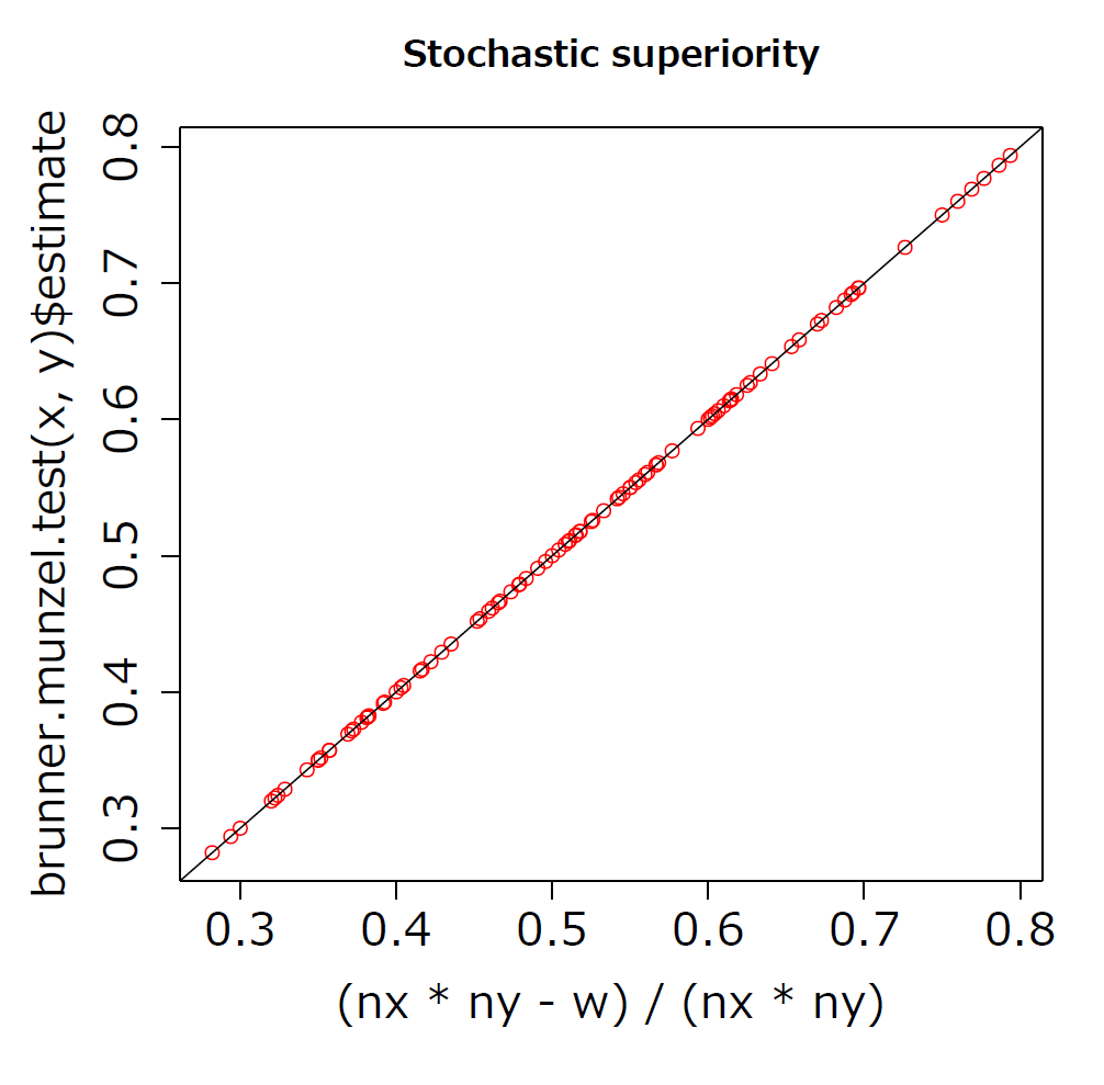
Mann-Whitney U 検定の検定統計量 W を使った定義による計算値(x 軸)と brunner.munzel.test 関数の estimate の数値が一致するのが分かる。
3. Brunner-Munzel 検定の効果量と Cohen's d の関係
実際に Stochastic superiority が用いられている例として,心理学的研究で Marmolejo-Ramos et al. (2013) p.7, Table 4 の下の説明を見てほしい。以下のように書かれている。
Measure of stochastic superiority (measure of effect size). The interpretation
benchmarks are: small, 0.56, medium, 0.64, and large, .71
これを良く知られた Cohen の d の効果量の基準(Cohen, 1992, p.157, Table 1)に対応させると,以下の表 1 のようになると考えられる。
この対応関係が実際に成り立つか,乱数データのシミュレーションで確認してみよう。
##################################
# シミュレーション

library(lsr)
library(lawstat)

p<- replicate(500, {

r<- runif(1, min = 0, max = 1)
x<- rnorm(100, mean = 0)
y<- rnorm(100, mean = r)

  c(
  # Cohen の d
  cohensD(x, y),

  # Brunner Munzel 検定効果量
  abs(brunner.munzel.test(x, y)$estimate - 0.5) + 0.5
  )
})

# グラフ
library(ggplot2)

dat<- data.frame(
   Cohens.d = p[1, ],
   Stochastic.superiority = p[2, ]
)

df.1 <- data.frame(
  x = c(-0.2, 0.2, 0.2, -0.2, 0.5, 0.5, -0.2, 0.8, 0.8),
  y = c(0.56, 0.56, 0, 0.64, 0.64, 0, 0.71, 0.71, 0),
  Effect.size = factor(rep(c(
    "small", "medium", "large"), each = 3
   ))
)

t.lab = c("0.2", "0.5", "0.8", "0.56", "0.64", "0.71")
x.lab = c(0.27, 0.57, 0.87, 0.02, 0.02, 0.02)
y.lab = c(0.4, 0.4, 0.4, 0.58, 0.66, 0.73)

g<- ggplot(dat, aes(
   Cohens.d, Stochastic.superiority)
   ) +
  geom_point() + theme_classic() +
  theme(text = element_text(size = 14)) +
  coord_cartesian(xlim = c(0, 1.5), ylim = c(0.4, 0.8))
g + geom_line(dat = df.1,
  aes(x = x, y = y, color = Effect.size), size = 1.2) +
  theme(legend.position=c(1, 1),
        legend.justification=c(1,1)) +
  annotate(
    "text",label = t.lab,
      x = x.lab, y = y.lab, size = 5)

#################
結果は,以下の図 2 のようになった。
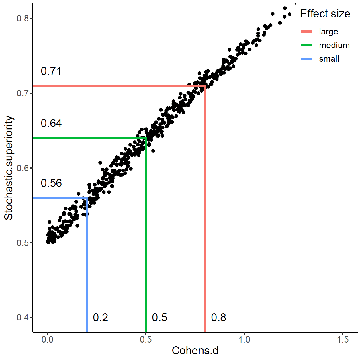
Brunner Munzel 検定効果量 Stochastic superiority が Cohen の d の大,中,小と対応関係にあることが分かる。
関連サイト
参考文献
Cohen, J. (1992) A power primer. Psychological Bulletin 112: 155–159.Marmolejo-Ramos, F., Elosúa, M. R., Yamada, Y., Hamm, N. F., and Noguchi, K. (2013) Appraisal of space words and allocation of emotion words in bodily space. PLoS One 8(12): e81688.