反復測定の比率データ: 一般化線形混合モデル ロジスティック回帰
井口豊(生物科学研究所,長野県岡谷市)
最終更新: 2022 年 12 月 6 日
1. はじめに
データ解析で,はい,いいえ
,のような二値変数の比率(正答率など)を分析する場合,一般化線形モデルのパラメトリック検定として,ロジスティック回帰分析が利用されることがある。
これが,2回,3回と,同じ物,同じ人に反復測定されることもある。そのような場合に使われるのが一般化線形混合モデル(generalized linear mixed model, GLMM)ロジスティック回帰分析である。
ここでは統計ソフト R を利用した例を示す。
2. 一般化線形混合モデルのロジスティック回帰分析
データは,テキストファイルで, test.dat としてダウンロードできる。
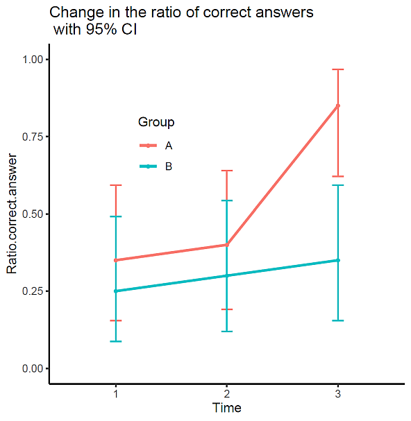
データ内容は 2 群 A, B で,各 20 人が, 3 回の検査を受け,正解(1)不正解(0)の結果を示したものである。
まず,その結果をまとめたグラフの R スクリプトである。
#############

# Data file
df<- read.table("test.dat", header=T)
head(df)

test<- c(df$test1, df$test2, df$test3)

dat<- data.frame(
  group = factor(rep(df$group, 3)),
  sub = factor(rep(df$sub, 3)),
  time = factor(rep(1:3, each = length(df$sub))),
  test = factor(test)
)

# Graph
#  CI lower limit
loci<- function(x) {
binom.test(c(length(x[x==1]), length(x[x==0])))$conf.int[1]
}

#  CI upper limit
upci<- function(x) {
binom.test(c(length(x[x==1]), length(x[x==0])))$conf.int[2]
}

r<- tapply(test, list(dat$group, dat$time), mean)

loci<- tapply(test, list(dat$group, dat$time), loci)
upci<- tapply(test, list(dat$group, dat$time), upci)

g.df<- data.frame(
  Time = factor(rep(1:3, each = 2)),
  Group = rep(c("A", "B"), 3),
  Ratio.correct.answer = as.numeric(r),
  CI.low = as.numeric(loci),
  CI.up = as.numeric(upci)
)

head(g.df)

library(ggplot2)

g<- ggplot(
  g.df,
  aes(
     x = Time, y = Ratio.correct.answer,
     color = Group, group = Group)
  ) +
  geom_line(size=1) +
  geom_errorbar(
     aes(ymin =  CI.low, ymax = CI.up),
         width = 0.1) +
  geom_point(size=1) +
  ylim(0, 1) +
  theme_classic() +
  theme(legend.position = c(0.3, 0.7)) +
  ggtitle(
   "Change in the ratio of correct answers \n with 95% CI"
  )

plot(g)

################
結果は,次の図 1 のとおりである。
このデータを一般化線形混合モデルのロジスティック回帰分析として計算する場合,例えば,以下のようなスクリプトができる。ただし,このモデル自体に柔軟性があるので,色々な変更が可能である。
#############
# GLMM logistic regression
mod<- glmer(test ~ time*group + (1 | sub),
   family = binomial(link="logit"),
   data = dat)

summary(mod)

################
結果は,固定効果だけ抜粋するが,以下のようになる。
Fixed effects:
                Estimate    Std. Error  z value  Pr(>|z|)
(Intercept)     -1.1517     0.8932  -1.289  0.19727
time2              0.3900     0.8865   0.440  0.65996
time3              4.2149     1.2953   3.254  0.00114 **
groupB           -1.2219     1.3736  -0.890  0.37367
time2:groupB   0.1321     1.3553   0.097  0.92233
time3:groupB  -3.2284     1.5747  -2.050  0.04035 *
3回目に有意に正答率が上がり,しかも,その時期と群との負の交互作用があって, B 群の変化が有意に小さくなっている,ことが分かる。
3. 一般化線形混合モデルを使った研究例
私が統計データ解析をサポートした五味志文さんの臨床研究では,一般化線型混合モデル(ガンマ分布)で分析した結果を示した。
五味志文(2022)
2 型糖尿病患者における経口セマグルチドの使用経験
—筋肉量と脂肪量の変化の検討—
Progress in Medicine 42(8): 77-82.
経口セマグルチド投与による筋肉量,HbA1c,体重,脂肪量の経時的変化を分析し,本剤が,筋肉量を減らさずに脂肪量を減少させ,高齢者でも有効に使えることを示唆している。